Yesterday, I finished Princeton’s course on Algorithms. The course can be found on Coursera, and it is an online version of the university’s on-campus introduction to algorithms and data structures. It is actually split in 2 parts on Coursera (Algorithms, Part I and Algorithms, Part II) that together form the equivalent of the on-campus course.

About the course

The first part starts with an introduction to the dynamic connectivity problem, and moves on to describing stacks and queues, sorting algorithms, and finishes with some more advanced data structures, such as the priority queue, balanced search trees and hash tables. The second one introduces graphs – both undirected and directed – and delves deeply into them. The problems of finding a minimum spanning tree and a shortest path are demonstrated, and graphs algorithms are finalized by the max flow and min cut problem. Subsequently, the course presents algorithms on strings; one of these – the one for regex searching – required building a nondeterministic finite automaton, which was probably the most advanced topic in the course. Finally, everything terminated with data compression!

The professor of the course was Robert Sedgewick, which was an amazing thing. He himself has devised some of the data structures taught in the course – such as red-black trees! And has completed a PhD supervised by Donald Knuth who is known as the “father of the analysis of algorithms”.

Assignments

Each part was 6 weeks, and had 5 assignments, meaning a total workload of 12 weeks and 10 assignments. The lectures were nice and had really cool visualizations that definitely helped in cementing the understanding. However, by far, the most brilliant part of the course were the assignments.

1. Percolation - a scary beginning

Honestly, seeing the first assignment was daunting. I even contemplated giving up on the course! We were expected to use the union find method presented in the lecture to answer whether a given system percolates:

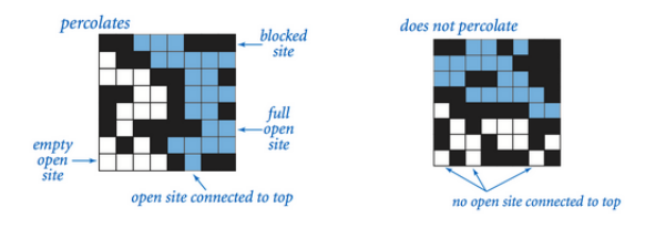
The sites (i.e., the blocks above) are opened randomly; and, after we have had made the algorithm to establish whether the system percolates, we had to estimate the percolation threshold for a given size, e.g. 20x20, using a Monte Carlo simulation! To be honest, it was the latter part that scared me, but in the end it turned out that finding whether a system percolates took me around 5-6 hours, following which writing the simulation actually was done in just 30-40 minutes.

Then, the assignment was to be submitted for automated feedback, where it is very extensively tested on different inputs, including randomly generated ones. The system was very helpful, because it provided suggestions and descriptions of what went wrong with each test, so often I would find myself submitting a “beta” version to see how well I’m progressing. Each submission is scored from 0-100, based on different criteria, such as correctness (60%), memory used (10%), timing (20%) and others. An assignment has “passed” if a score of over (or exactly) 80% is achieved.

My very first submission resulted in 75% which definitely made me happy! The grader showed a lot of tests passing, and some failing. The latter were due to a bug, which I quickly identified and just 20 minutes later I had passed my first assignment with a grade of 94%!

At first, I actually planned to just leave it there; especially because the missing 6% were from a bug called backwashing that was actually mentioned in the assignment FAQ:

[i]t is only a minor deduction (because it impacts only the visualizer and not the experiment to estimate the percolation threshold), so don’t go crazy trying to get this detail.

And, indeed I left it as it was… for a day. It was bugging me, knowing that I can improve further, so on the next day, I spent an extra hour improving the performance, and fixed the backwashing! My submission then resulted in a 98%, with the 2% missing for using a sub-optimal implementation for the backwashing problem fix.

Still, since I wanted to finish the course while the COVID-19 lockdown is going on, I decided not to be a perfectionist and move on with 98 out of 100 points!

2. Queues - picking up speed

Strangely, I found the second assignment to be easier – we had to build a double-ended queue (deque) – i.e., a stack and a queue together (adding and removing things from both sides possible), and a randomized queue – which, evidently from the name, removes a random item from the data structure. With some 7-8 hours of work, I managed to get a score of a 100!

3. Collinear points & 4. Slider Puzzle - I wrote pattern recognition & AI search algorithms!

Then, two very interesting assignments followed: collinear points, where I implemented a basic version of pattern recognition – finding a subset of 4 or more points on the same line segment. This was the first time I did something related with computational geometry, and also the first for using generics in Java, as well as the Comparable interface. Since the course actually expected us to know the idea of generics, I had to do some reading on my own for it. Luckily, it didn’t take me much time, as I found the idea quite straightforward. Ultimately, I got another 98% for this assignment!

The next assignment was also very cool, as mentioned above: I implemented an AI algorithm called A* search from scratch! The assignment was to design a 8-puzzle solver. Checkout the assignment link if you are not familiar with 8-puzzle (as was the case for me). We also had to create two priority functions for our algorithm, using different notions of distance – the Hamming, and Manhattan distance. This one was another 100/100 for me!

5. KD-Trees - in my MSc, I used the k-nearest neighbors algorithm; here, I wrote it!

I finished part one of the course by building a kd-tree. This was one hard assignment! It took me a full day of work (7-8 hours) to get to a submit-worthy version. It resulted in 77 points – so close! Still, I called it a day and it wasn’t until next morning that I got an 85 – passed! Of course, this wasn’t enough for me :) I spent extra 5 hours on that Sunday optimizing my solution and got the holy 100 points! To be fair, I’m not sure if I’d like to spend a normal weekend doing this, but it’s not like I had any plans with the whole COVID-19 thing going on. However, I am definitely glad I did this: kd-trees showed me how to implement the nearest-neighbor search! I studied about this algorithm in my university class on big data analytics, but there we just took it as a given (i.e., a blackbox) and focused on its business applications (as, of course, is expected at a Business school). But finding out how things work under the hood feels great!

6. WordNet

The first part of the course terminated with a lecture-only week that introduced hash tables, and part 2 continued with graphs! First assignment was to build a shortest ancestral path for words. An ancestor is a hypernym; for example, run is a hypernym (ancestor) of sprint. Since this structure required us to work with a very specific type of graph – a directed acyclic graph (DAGs), I actually (relatively) quickly devised a solution and submitted, only to find out we were tested on not just DAGs, but any digraphs (which to be fair was mentioned in the FAQ, but I apparently missed it). So my first submission didn’t score too well, but with a few extra hours, I managed to generalize it to work for any digraph… and got another 100!

7. Seam Carving - I wrote a recently-discovered algorithm used in Photoshop!

Warning: this section contains some light spoilers about the assignment solution.

The following assignment was my favorite. We implemented an algorithm that is used by Photoshop for content aware resize of images, called seam carving. You can check out the idea behind it here:

Actually, this algorithm is quite new – discovered only in 2007! The way we were supposed to apply it was by treating the image as a digraph of pixels (each connected to the bottom ones), and making a topological sort of the pixels. The weights of the digraph edges are the “energy” of the pixels, as described in the video. I actually couldn’t wrap my head around how to apply the topological sort in this scenario, but I figured something else: since we want the shortest path to the bottom, if we look at the picture in a reverse order: i.e., starting from the bottom pixels, we can take advantage of something very important. Let's illustrate it with an example: by specification, the bottom pixels all have an energy of 1000 (as well as all other border pixels):

And, let’s assume that the pixels from the row above the bottom have the following (made-up) values:

Meaning that as of now, we have the following last 2 rows:

Here’s the image with an extra row with no energies added (as we don’t need them to see what I’m saying). We are focusing on the highlighted in red pixel:

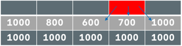
The blue arrows are the edges in our (implicit) graph. So, without needing to know anything extra, we can immediately see what would be the shortest path from this pixel to the bottom: take the left pixel and then any of its adjacent ones (doesn’t matter which one exactly because all 3 of its adjacent are at the bottom and thus have an energy of 1000). So, by generalizing this idea and scanning the image from the bottom, and saving the “shortest distance to bottom” for each pixel (e.g., the shortest distance to bottom for our red pixel above is 600 + 1000 = 1600), by the time I finish scanning the pixels, I already know the shortest path to the bottom! To be fair, the assignment FAQ states the following:

Can I use dynamic programming? Yes, though, in this context, dynamic programming is equivalent to the topological sort algorithm for finding shortest paths in DAGs.

So, I am assuming that this relates to my situation. Anyway, once this was done, I had solved most of the task! What was left was to make some optimizations, such as re-calculating the energies of only the affected pixels after removing a seam (i.e., not rescanning the whole image from scratch). This was done, and… I got another 100!

8. Baseball Elimination & 9. Boggle - finishing up graph problems!

In one of the lectures, professor Sedgewick let us know that apparently sport journalists are not too good at algorithms, and, as a result, they would often report wrong baseball standings! I.e., a baseball standing is supposed to show which teams still have a chance of winning the title – meaning, to finish first, and which not – meaning, they are eliminated. Of course, getting the so-called trivial eliminations is easy – if team A has 70 wins and 10 games left, and team B has 55 wins and 10 games left, it’s pretty clear that team B is eliminated. But there are more tricky situations, where it might appear that a team has a chance of catching up if they win all their games left, but the scheduling of the remaining games makes it so that they are still eliminated. Apparently, this translates perfectly to a maxflow/min cut problem, so this was the assignment: take a baseball division as an input, and determine which teams are eliminated! It wasn’t my favorite assignment of the course, but still, solved it and managed to get a 100!

The next one, I liked much better! We had to create a Boggle solver. Again, check out the link for explanation of the game. It is kind of a Sudoku / Scrabble combination. It was fun because, unlike in the other assignments, we didn’t have much limitations with regards to the amount of memory we can use; instead, pure speed was the goal! Figuring this out in my head was quite tricky; especially because we had to solve a problem which was very well-suited for a graph, but, to make things faster, it was suggested to work with an implicit graph. I.e., there was no actual graph, but we had to write a code that would work on the given Board data structure (a 2d array), as if it was a graph! So, writing the depth first search was quite tricky. Not only this, but we had a special character – the letters ‘Q’ and ‘U’ were appearing together as ‘Qu’, so we also had to handle this case. Still, some 10 hours of work resulted in a cool 100 points!

10. Burrows–Wheeler - outcompressing gzip!

The last assignment had us writing the first 2 of the 3 steps of the Burrows–Wheeler data compression algorithm:

1. Burrows–Wheeler transform: given a file, transform it into one where sequences of the same character occur near each other many times;
2. Move-to-front encoding: given the file from above, transform it to a file where certain characters appear much more frequently than others;
3. Huffman compression

We worked a lot with binary data, which for me proved relatively easy, mainly thanks to David Malan’s fantastic explanations in CS50. Overall, it took me only around 7 hours, which surprised me, as I was expecting something crazy-difficult as an ending assignment. Also, what the professors called “the trickiest part conceptually”, I didn’t spend much time at. On the other hand, the move-to-front encoding, which I was expecting to be trivial, turned out the trickiest for me. And, on top of that, for a seemingly very simple operation – moving in a sequence of variables, for example:

1. Starting state of sequence: A B C D E
2. Next state of sequence: C A B D E

Notice something crucial: this is not swapping! If we were to simply swap C and A, well, that’s obviously a first-programming-course level difficulty. However, again, this is not the case, as we are moving the variable; i.e., in this example, B is also affected. I spent some time thinking what would be the best data structure for this, and honestly, couldn’t come up with a perfect solution. What I ended up with was an ArrayList, that I would scan until I found the character I’m looking for, remove it, and then add it at index 0. It definitely didn’t feel optimal to me, but it was the best I got.

After submitting, the grader suggested that an array might be better for performance, but I really couldn’t see how – the shifting operation would be very expensive, IMO. Anyway, despite all this, I passed all 38 timing tests for the move-to-front part! So, apparently, this was a good solution.

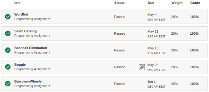
Actually, on this last assignment, I got my highest score on first submit – a whooping 97 points!! In fact, just a few minutes later, I got a 99 – I had lost 2 points, because I failed to consider a corner case – words that are nontrivial circular suffixes of themselves, e.g. ************. So, this was a quick bugfix. Then, another hour and a half tuning the performance, and… 100 points!!! I wanted to get those, so that I can have the second part finished with all assignments with 100%, and I did it:

Closing notes

Overall, this has been an extremely brilliant course, and I am very grateful to professors Robert Sedgewick and Kevin Wayne for providing it completely for free. I would recommend it to anyone that has already mastered the fundamentals of CS (i.e., as a fourth or fifth CS course). You also do not need to know Java to take it. The community is great, and still active, years after the start of the course! There’s also enough official support, from mentors of the course, which are volunteer past-students (actually, the most active one is also a Bulgarian!). So, I would say that this course is comparable to CS50 in quality, which is a great compliment!